Improving xumx-sliCQ (slightly)

Introduction

In 2021, I created xumx-sliCQ. It's a neural network for music demixing, or music source separation:

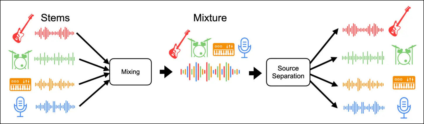
Music demixing systems take in a mixed pop song - mixed meaning the final version with all instruments and vocals combined - as an input, and output an estimation of isolated sources. During the time frame that I worked on the problem (2021), the dominant dataset was MUSDB18-HQ, which includes the mixed song and four stems (vocals, drums, bass, other). Some examples are Open-Unmix, Spleeter, and Demucs. My own example is xumx-sliCQ.

xumx-sliCQ

My first As a starting point, I took a baseline model, Open-Unmix (or UMX) and applied the cross-target modifications from CrossNet-Open-Unmix (or X-UMX). Then, I replaced its spectral transform with a different one. UMX uses the ubiquitous Short-Time Fourier Transform (STFT), while my plan involved the Nonstationary Gabor Transform (NSGT), or its variant designed for varying signal lengths, the Sliced Constant-Q Transform (sliCQT).

My hypothesis was that without requiring dramatic changes to the network architecture, using a spectral transform with more musical information would improve the results magically. In the end, xumx-sliCQ fell far short of my expectations, scoring 3.6 dB on the standard benchmark compared to the 5+ dB scores of UMX and X-UMX. For reference, current state-of-the-art models such as Demucs score around 9 dB these days (2023).

I came at xumx-sliCQ the "hard way", using a transform that other people have not used in a neural network before. I persisted and it seemed to take me the effort of a lifetime to get something even remotely passable: I preserved 31 total failed experiments, although were likely more. I don't know if disciplined deep learning practitioners do some careful statistical analysis of the data and run smaller experiments before trying to create and train an entire architecture to test a hunch. In my case, I definitely applied the "grad student descent" algorithm:

For example, to work with a neural network you have to choose the number of layers, the weight regularization, the layer size, which non-linearity, the batch size, the learning rate schedule, the stopping conditions… How do people choose these parameters? Mostly with ad hoc, black magic methods.
One method, common in academia, is ‘grad student descent’ (a pun on gradient descent), in which a graduate student fiddles around with the parameters until it works. - https://sciencedryad.wordpress.com/2014/01/25/grad-student-descent/

I can dispute whether my expectations were reasonable in the first place; I, a fresh grad student, to whom music demixing (and audio/music signal processing in general) was merely a GitHub/open-source hobby, and a newbie to machine learning and deep learning to boot, expected to stride in and beat the near-state-of-the-art with a magical idea nobody had yet thought to do?

I could try to reframe my achievement as "successfully implemented a neural network using a brand new paradigm of spectral transform," wherein a lot of parameters and different architectures are now made possible. However, I don't think the person who's going to make a world-beating music demixing system is eyeballing 3.6 dB solutions as their starting point.

I told myself after xumx-sliCQ that I was done with open-source projects:

2022 is when I'm no longer overtly interested in dramatic bouts of hard work or burning the candle.

Here's the story of how I ruined the beginning of my 2023 by breaking my promise and working on xumx-sliCQ-V2.

Unreasonable expectations

Nobody works on things for modest improvements. It's a waste of time. The only justification I have for putting so much work into crap like xumx-sliCQ is that I truly believe I would come out the other end victorious; achieving some watermark of quality, performance, efficiency, or all of the above. Of course, what ends up happening in reality is perhaps a modest achievement: solid, something to be proud of in the context of my own life and abilities, but not world-beating, certainly not on my first try.

I (felt that I) knew that xumx-sliCQ had enormous potential; after all, it's the perfect middleground between STFT-based models and waveform-based models! My take on Gabor's time-frequency uncertainty principle is this:

• Choosing a fixed window size to generate the time-frequency domain STFT of a time-domain waveform ( results means a tradeoff in time or frequency resolution (this is known)
• Operating directly on the time-domain waveform avoids this issue
• Operating on waveforms is difficult (only popular recently), and in practice time-frequency transform representations are often used in audio or music neural networks

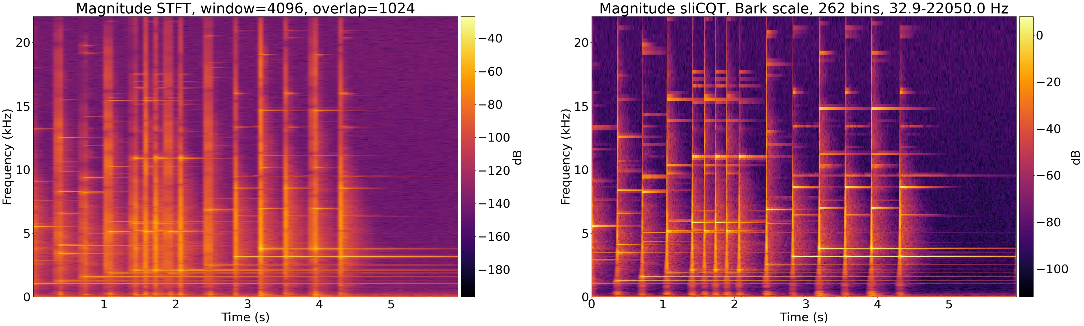
What makes the sliCQT special? It can be designed to analyze sound with any arbitrary monotonically-increasing frequency scale. Instead of choosing a fixed window size, you can instead decide what frequency spacing you want, following the nonlinear model of human hearing/psychoacoustics; you can create a set of finely spaced frequency bins in the low frequency regions, and coarse frequency bins in the high frequency regions, to get the best of both worlds: good frequency information in the harmonic regions, and good temporal information in the percussive/transient regions:

Creation of xumx-sliCQ-V2: roadmap

My initial modifications to the code of xumx-sliCQ were efforts to speed up the epochs. Epochs are the iterations during which a neural network is trained: in each epoch, the network is shown a new batch of data while it adjusts its parameters to generate better results. The faster the epochs, the more experiments and iterating I can do (hyperparameter tuning, etc.) Also, over the past year I had become aware of a performance tuning guide for PyTorch with some CUDA-specific tricks that I wanted to incorporate.

The plan shaping up in my head was:

• Make code more efficient and tuned wherever possible to make epochs faster
  • Eliminate sloppy or duplicate computations
  • Eliminate unnecessary copies between host and device (CPU and GPU) during training
  • Add special flags/features/performance tuning targeted for Torch and CUDA
• When epochs are as fast as possible, iterate on the neural network architecture until the performance improves

Docker setup with nvidia-docker2

In the old codebase of xumx-sliCQ, I failed to provide a reproducible Python development environment; due to having unpinned dependencies and relying on the current state/latest version of libraries and packages available on the Fedora repos at the time that I was working on it, it was not easy at all for me to revisit it later and get it running. I also used a mix of pip and conda without understand their interactions with one another. Imagine, if the creator had trouble reproducing their own work, how hard it would be for newcomers?

With xumx-sliCQ-V2, I started using Docker with nvidia-docker2, especially after learning that NVIDIA hosts variants of popular deep learning framework images that come preloaded with optimizations out-of-the-box. I based the Docker image for xumx-sliCQ-V2 on the NVIDIA PyTorch container.

In the project's Dockerfile, these three lines are very useful:

COPY . /xumx-sliCQ-V2
WORKDIR /xumx-sliCQ-V2
RUN python -m pip install -e .

What this does is:

1. Copy the source code of xumx-sliCQ-V2 into the container at /xumx-sliCQ-V2
2. Install it in pip editable mode such that the xumx_slicq_v2 module in the container's Python interperter uses code that's dynamically symlinked to /xumx-sliCQ-V2
3. This way, you can either run the image to use xumx_slicq_v2 code copied at image build time, or you can bind a volume with modified source code on your host to the container to use your local code changes: -v /home/sevagh/repos/xumx-sliCQ-V2:/xumx-sliCQ-V2
4. With volume mounts, I can do other neat tricks to simplify the code, like mounting the dataset to /MUSDB18-HQ, or mounting a local path to save a model -v /path/to/save/model:/model (vs. allowing the model being trained at /model to be discarded by only saving it to the Docker volume)

Another neat advantage is that we can strictly separate GPU and CPU scripts by not providing the docker run commands with any GPUs:

1. Run GPU training to produce ./trained-model:

   docker run --rm -it \
       --gpus=all --ipc=host --ulimit memlock=-1 --ulimit stack=67108864 \ # recommended GPU settings
       -v /home/sevagh/Music/MUSDB18-HQ/:/MUSDB18-HQ \ # dataset volume mount
       -v /home/sevagh/repos/xumx-sliCQ-V2/:/xumx-sliCQ-V2/ \ # local source code
       -v /home/sevagh/repos/xumx-sliCQ-V2/trained-model/:/model \ # persist local model
       -p 6006:6006 \ # ports for tensorboard or optuna web dashboards
       xumx-slicq-v2 \
       python -m xumx_slicq_v2.training \
       --batch-size=64 --nb-workers=8 --debug # training CLI args
   

2. Simultaneously run a CPU evaluation on ./trained-model without worrying about accidentally using the GPU and interfering with the running training process:

   docker run --rm -it \
       -v /home/sevagh/Music/MUSDB18-HQ/:/MUSDB18-HQ \ # dataset volume mount
       -v /home/sevagh/repos/xumx-sliCQ-V2/:/xumx-sliCQ-V2/ \ # local source code
       -v /home/sevagh/repos/xumx-sliCQ-V2/trained-model/:/model \ # persist local model
       xumx-slicq-v2 \
       python -m xumx_slicq_v2.evaluation \
       --model-path="/model" --track='Zeno Signs' # evaluation CLI args
   

Code optimizations

Eliminating CPU-GPU copies between torch tensors and numpy ndarrays

This part is sloppy so bear with me:

• xumx-sliCQ contains code to generate the sliCQT inside it
• That code is based on original NumPy code that I transliterated to PyTorch
• The copy in xumx-sliCQ is equivalent and maintains parity with my standalone fork of the original numpy code, released so that people can work on other PyTorch applications that use the NSGT/sliCQT outside of xumx-sliCQ
• In xumx-sliCQ-V2, I copied it yet again to make new changes described in this section

The training and neural network code of xumx-sliCQ was copied from the PyTorch implementation of open-unmix, so there was a low chance of accidental CPU-GPU transfers. However, the sliCQT code, containing my own imperfect transliteration from NumPy to PyTorch, could indeed be full of sloppy leftover numpy ndarrays.

buildah bud -t "xumx-slicq-v1" --build-arg CLONE_V1=yes .

podman run --rm -it --ipc=host --gpus=all \
    -v /home/sevagh/Music/MDX-datasets/MUSDB18-HQ/:/MUSDB18-HQ \
    xumx-slicq-v1  \
    python /xumx-sliCQ/scripts/train.py \
        --batch-size=64 --nb-workers=8 --debug --root=/MUSDB18-HQ'

When observing GPU usage from nvtop while training the old v1 code, the telltale signs of wasteful host-device (or CPU-GPU) transfers are spiking Tx/Rx (transmitted and received) data as well as low (and fluctuating) GPU usage:
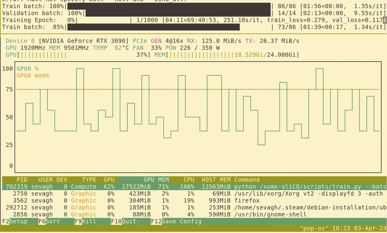Note the GPU usage hovering between 30ish and 80ish %.

After eliminating all accidental/leftover usages of numpy in the middle of the torch training loop that I could find, the GPU usage got much higher, hovering near 75% with rare drops to 50%:

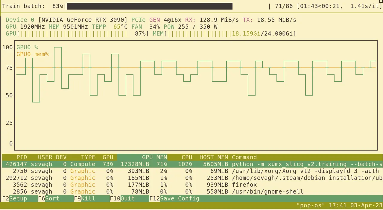
Aside from text searches for np. and numpy, I found another tool for debugging any sneaky numpy CPU ndarrays that were causing host-device transfers in the training loop; a tip from the PyTorch forums to debug tensor devices from gc (Python's garbage collection module).

Python function:

import gc
import torch

def check_tensors_devices(prefix):
    count_cpu_tensors = 0
    count_gpu_tensors = 0
    count_cpu_tensors_with_grad = 0
    count_gpu_tensors_with_grad = 0
    for obj in gc.get_objects():
        try:
            if torch.is_tensor(obj) or (hasattr(obj, 'data') and torch.is_tensor(obj.data)):
                if obj.device == torch.device("cpu"):
                    count_cpu_tensors += 1
                    if obj.requires_grad:
                        count_cpu_tensors_with_grad += 1
                elif obj.device == torch.device("cuda:0"):
                    count_gpu_tensors += 1
                    if obj.requires_grad:
                        count_gpu_tensors_with_grad += 1
        except:
            pass
    print(f"{prefix} CPU TENSORS: {count_cpu_tensors}, WITH GRAD: {count_cpu_tensors_with_grad}")
    print(f"{prefix} GPU TENSORS: {count_gpu_tensors}, WITH GRAD: {count_gpu_tensors_with_grad}")
    print()

Then add calls to check_tensor_devices to investigate your code:

def loop(...):
...
        check_tensors_devices("A")
        x = track_tensor_gpu[:, 0, ...]
        check_tensors_devices("B")
        # forward call to unmix returns bass, vocals, other, drums
        estimates_waveforms = unmix(x)
        check_tensors_devices("C")
        loss = criterion(
            estimates_waveforms, # estimated by umx
            track_tensor_gpu[:, 1:, ...], # target
        )
        check_tensors_devices("D")

    if train:
        check_tensors_devices("E")
        optimizer.zero_grad()
        check_tensors_devices("F")
        loss.backward()
        check_tensors_devices("G")
        optimizer.step()
        check_tensors_devices("H")

General inefficiencies: list-of-tensors vs. the Nested Tensor

The sliCQT, as it appears in my project, is a ragged list of tensors (i.e. a list of tensors of different length):

# STFT shape
print(stft_spectrogram.shape, stft_spectrogram.dtype)
(1, 2, 2049, 47), torch.complex64

# 1 = batch size
# 2 = number of channels (stereo)
# 2049 = number of non-redundant frequency bins (4096//2+1)
# 47 = number of time frames

# sliCQT shape
for tf_block in slicqt:
    print(tf_block.shape, tf_block.dtype)

# first 86 frequency bins at the lowest time resolution (100 frames)
(1, 2, 86, 100)

# next 4 frequency bins at 160 frames
(1, 2, 4, 160)

# next 2 at 192 frames (note the increasing time resolution)
(1, 2, 2, 192)

# last frequency bin at the highest time resolution (238 frames)
(1, 2, 1, 238)

Also, note that there are 4 identical sub-neural networks, for the 4 targets (vocals, drums, bass, other). This is how the neural network was set up in xumx-sliCQ:

self.nn_vocals = []
self.nn_drums = []
self.nn_bass = []
self.nn_other = []

for tf_block in slicqt:
    # initialize a neural network per time-frequency block

    # use each block's size to dynamically define the neural network params
    self.nn_vocals.append(OpenUnmixCDAE(tf_block))
    self.nn_drums.append(OpenUnmixCDAE(tf_block))
    self.nn_bass.append(OpenUnmixCDAE(tf_block))
    self.nn_other.append(OpenUnmixCDAE(tf_block))

In this example, for each time-frequency block in the sliCQT, the following operation is repeated:

def forward(x):
    # input = x = mixed song

    mix = x.detach().clone()

    # nn code to compute mask
    x = self.layer1(x)
    x = self.layer2(x)
    ...

    return x*mix

Due to the list-of-tensors datastructure, although this seems like a small inefficiency, the effect multiplies for each time-frequency block.

In xumx-sliCQ-V2, I revisited the issue to eliminate these redundancies, working with a list-of-tensors datastructure better than before:

self.nn_all_targets = []

for tf_block in slicqt:
    # initialize a neural network per time-frequency block

    # use each block's size to dynamically define the neural network params
    self.nn_all_targets.append(OpenUnmixCDAE(tf_block))

# each sub-neural-network has four separate stacks of layers

class OpenUnmixCDAE:
...
def __init__(self, tf_block):
    layer1 = Conv2d(...)
    layer2 = Conv2d(...)
    self.layer1s = [copy.deepcopy(layer1) for i in range(4)]
    self.layer2s = [copy.deepcopy(layer2) for i in range(4)]
    ...

def forward(x):
    # input = x = mixed song

    mix = x.detach().clone()

    # store 4 outputs for 4 targets
    ret = torch.zeros((4, *mix.shape))

    # nn code to compute mask
    for i in range(4):
        x_tmp = x.clone()
        x_tmp = self.layer1s[i](x_tmp)
        x_tmp = self.layer2s[i](x_tmp)
        ...

        ret[i] = x_tmp*mix

    return ret

I didn't measure each little win in isolation, but having better, cleaner, more efficient code makes me happier even without any measured impact.

I thought the Nested Tensor, ragged/jagged tensors for PyTorch, would help, but they're pretty limited. I can't even do torch.abs(nested_tensor)! Which, for me, defeats the purpose. Woudln't you think it's trivial to support this operation?

nested_tensor = [(2, 3), (4, 5), (6, 7)] # arbitrary collection of shapes
abs_nested_tensor = torch.abs(nested_tensor) # why not??

# instead i'm forced to do this
list_of_tensors = [(2, 3), (4, 5), (6, 7)]
abs_list_of_tensors = [torch.abs(t) for t in list_of_tensors]

Although the nuts and bolts of the underlying neural network would have been difficult to code, owing to the complexity of the sliCQT's ragged nature, supporting basic operations like magnitude, phase, addition, multiplication, etc. on nested tensors would have gone a long way in making the code of xumx-sliCQ much more readable and efficient. As it stands, I don't know what the point is of a nested tensor API that can't do any tensor operations at all.

PyTorch/CUDA performance tuning

I first started with the easiest step: simply use the NVIDIA PyTorch container.

The NVIDIA container automatically enables optimizations like TensorFloat-32 aka TF32. However, there are further optimizations that need to be enabled by code, from the PyTorch performance tuning guide:

######################
# PERFORMANCE TUNING #
######################
print("Performance tuning settings")
print("Enabling cuDNN benchmark...")
torch.backends.cudnn.benchmark = True

print("Enabling FP32 (ampere) optimizations for matmul and cudnn")
torch.backends.cudnn.allow_tf32 = True
torch.backends.cuda.matmul.allow_tf32 = True
torch.set_float32_matmul_precision = "medium"

print(
    "Enabling CUDA+CPU Automatic Mixed Precision with for forward pass + loss"
)

# lstm can only support float16 optimizations
cuda_autocast_dtype = torch.bfloat16 if not args.lstm else torch.float16
amp_cm_cuda = lambda: torch.autocast("cuda", dtype=cuda_autocast_dtype)

amp_cm_cpu = lambda: torch.autocast("cpu", dtype=torch.bfloat16)

Automatic Mixed Precision training, casting down to BFloat16, saves a lot of memory and allows bigger batch sizes. In practice, I didn't notice the loss of precision influencing the music demixing results in any way; this is a straight upgrade.

The rest, like "disable bias in conv before batch norm," are things I've already been using in xumx-sliCQ since the V1 code:

encoder.extend([
    Conv2d(
        hidden_size_1,
        hidden_size_2,
        (freq_filter, time_filter_2),
        bias=False,
    ),
    BatchNorm2d(hidden_size_2),
    ReLU(),
])

An epoch takes ~170s (train + validation) on my RTX 3090 with 24GB of GPU memory with --batch-size=64 --nb-workers=8. xumx-sliCQ by contrast took 350s per epoch with a batch size of 32 on an RTX 3080 Ti (which had 12GB GPU memory, half of my 3090). However, the old code used PyTorch 1.10, so the upgrade to the prerelease 1.14 version of PyTorch may also be contributing to the improved performance.

However, I suggest you read the entire guide to ensure you're not leaving any easy performance wins on the table.

Trusting my own code

At some point, I wasted time trying to get a poorly-designed library to help me work on xumx-sliCQ (for faster BSS evaluations). After opening multiple issues and getting nothing useful and usable, I remembered that I had my own fast GPU-accelerated BSS fork that I used for xumx-sliCQ.

Moral of the story: I'd rather trust my own code because I know that it works the way I advertise it on the README.

Paying for Git-LFS

Another simple enhancement to my quality of life while iterating on xumx-sliCQ-V2 was paying for a GitHub LFS data pack. Git LFS is git's Large File Storage. I was able to store many copies of my trained weights (torch .pth files) for a pretty low price ($4 USD per month). Totally worth the improved workflows and reproducibility without worrying about how many pth files I could train and store.

Successful changes (from 3.6 dB to 4.4 dB)

The SDR score (signal-to-distortion ratio, which is the predominant single quantitative score used to rank a system's music demixing performance) went from 3.6 dB (in the old V1 code) to 4.4 dB as a result of these changes. Most of this is copied from the project README.

Using the full frequency bandwidth

In xumx-sliCQ, I didn't use frequency bins above 16,000 Hz in the neural network; the demixing was only done on the frequency bins lower than that limit, copying the umx pretrained model of UMX. UMX's other pretrained model, umxhq, uses the full spectral bandwidth. In xumx-sliCQ-V2, I removed the bandwidth parameter to pass all the frequency bins of the sliCQT through the neural network.

Removing dilations from the convolution layers

In the CDAE of xumx-sliCQ, I used a dilation of 2 in the time axis to arbitrarily increase the receptive field without paying attention to music demixing quality (because dilations sound cool).

In xumx-sliCQ-V2, I didn't use any dilations since I had no reason to.

Removing the inverse sliCQT and time-domain SDR loss

In xumx-sliCQ, I applied the mixed-domain SDR and MSE loss of X-UMX. However, due to the large computational graph introduced by the inverse sliCQT operation, I was disabling its gradient:

X = slicqt(x)
Xmag = torch.abs(X)
Ymag_est = unmix(Xmag)
Ycomplex_est = mix_phase(torch.angle(X), Ymag_est)

with torch.no_grad():
     y_est = islicqt(Ycomplex_est)

Without this, the epoch time goes from 1-5 minutes to 25+ minutes, making training unfeasible. However, by disabling the gradient, the SDR loss can't influence the network performance. In practice, I found that the MSE was an acceptable correlate to SDR performance, and dropped the isliCQT and SDR loss calculation.

Replacing the overlap-add with pure convolutional layers

A quirk of the sliCQT is that rather than the familiar 2 dimensions of time and frequency, it has 3 dimensions: slice, time-per-slice, and frequency. Adjacent slices have a 50% overlap with one another and must be summed to get the true spectrogram in a destructive operation (50% of the time coefficients are lost, with no inverse).

In xumx-sliCQ, an extra transpose convolutional layer with stride 2 is used to grow the time coefficients back to the original size after the 4-layer CDAE, to undo the destruction of the overlap-add.

In xumx-sliCQ-V2, the first convolutional layer takes the overlap into account by setting the kernel and stride to the window and hop size of the destructive overlap-add. The result is that the input is downsampled in a way that is recovered by the final transpose convolution layer in the 4-layer CDAE, eliminating the need for an extra upsampling layer.

Diagram (shown for one time-frequency block):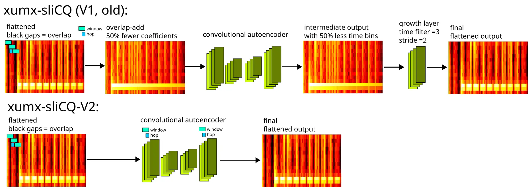

By this point, I had a model that scored 4.1 dB with 28 MB of weights using magnitude MSE loss.

Differentiable Wiener-EM and complex MSE

Borrowing from Danna-Sep, one of the top performers in the MDX 21 challenge, the differentiable Wiener-EM step is used inside the neural network during training, such that the output of xumx-sliCQ-V2 is a complex sliCQT, and the complex MSE loss function is used instead of the magnitude MSE loss. Wiener-EM is applied separately in each frequency block as shown in the architecture diagram at the top of the README.

This got the score to 4.24 dB with 28 MB of weights trained with complex MSE loss (0.0395).

In xumx-sliCQ, Wiener-EM was only applied in the STFT domain as a post-processing step. The network was trained using magnitude MSE loss. The waveform estimate of xumx-sliCQ combined the estimate of the target magnitude with the phase of the mix (noisy phase or mix phase).

Discovering hyperparameters with Optuna

Using the included Optuna tuning script, new hyperparameters that gave the highest SDR after cut-down training/validation epochs were:

• Changing the hidden sizes (channels) of the 2-layer CDAE from 25,55 to 50,51 (increased the model size from ~28-30MB to 60MB)
• Changing the size of the time filter in the 2nd layer from 3 to 4

Note that:

• The time kernel and stride of the first layer uses the window and hop size related to the overlap-add procedure, so it's not a tunable hyperparameter
• The ragged nature of the sliCQT makes it tricky to modify frequency kernel sizes (since the time-frequency bins can vary in their frequency bins, from 1 single frequency up to 86), so I kept those fixed from xumx-sliCQ
• The sliCQT params could be considered a hyperparameter, but the shape of the sliCQT modifies the network architecture, so for simplicity I kept it the same as xumx-sliCQ (262 bins, Bark scale, 32.9-22050 Hz)

This got the score to 4.35 dB with 60 MB of weights trained with complex MSE loss of 0.0390.

Mask sum MSE loss

In spectrogram masking approaches to music demixing, commonly a ReLU or Sigmoid activation function is applied as the final activation layer to produce a non-negative mask for the mix magnitude spectrogram. In xumx-sliCQ, I used a Sigmoid activation in the final layer (UMX uses a ReLU). The final mask is multiplied with the input mixture:

mix = x.clone()

# x is a mask
x = cdae(x)

# apply the mask, i.e. multiplicative skip connection
x = x*mix

Since the mask for each target is between [0, 1], and the targets must add up to the mix, then the masks must add up to exactly 1:

drum_mask*mix + vocals_mask*mix + other_mask*mix + bass_mask*mix = mix
drum_mask + vocals_mask + other_mask + bass_mask = 1.0

In xumx-sliCQ-V2, I added a second loss term called the mask sum loss, which is the MSE between the sum of the four target masks and a matrix of 1s. This needs a small code change where both the complex slicqt (after Wiener-EM) and the sigmoid masks are returned in the training loop.

This got the score to 4.4 dB with 60 MB of weights trained with complex MSE loss + mask sum loss of 0.0405.

Realtime variant

For a future realtime demixing project, I decided to create a realtime variant of xumx-sliCQ-V2. To support realtime inputs:

• I added left padding of the first convolution layer, such that the intermediate representations throughout the autoencoder are only derived from causal inputs
• I replaced the resource-intensive Wiener-EM target maximization with the naive mix-phase approach, which is computationally much lighter (simply combine the target magnitude slicqt with the phase of the mix)

Final results

The scores achieved by the improved models of xumx-sliCQ-V2 were:

• 4.4 dB on the offline model
• 4.1 dB on the realtime model

These were improvements over the 3.6 dB scored by the first model, although the model more than doubled in size (60MB is still nothing compared to the multi-GB sizes of top-quality models).

Ragged spectrograms

I added code to generate spectrograms for the ragged sliCQT. With the old xumx-sliCQ code, I preserved the matrixform option of the sliCQT, which has zero-padding somewhere in the transform (though not naively stuffing zeros to the right of the smaller frequency bins; the zero-padding is done before the FFT/iFFT of the ragged intermediate structures). The matrixform allows for simple rectangular spectrograms to be plotted.

In xumx-sliCQ-V2, I ditched the matrixform entirely, leaning on the ragged list-of-tensors. Therefore, I need to generate a ragged list-of-spectrograms to represent a signal. The script:

podman run --rm -it \
    -v /home/sevagh/Music/MDX-datasets/MUSDB18-HQ/:/MUSDB18-HQ \
    -v /home/sevagh/repos/xumx-sliCQ-V2:/xumx-sliCQ-V2 \
    -v /home/sevagh/repos/xumx-sliCQ-V2/plots:/spectrogram-plots \
    xumx-slicq-v2 \
    python -m xumx_slicq_v2.visualization

Example (resized and stacked together):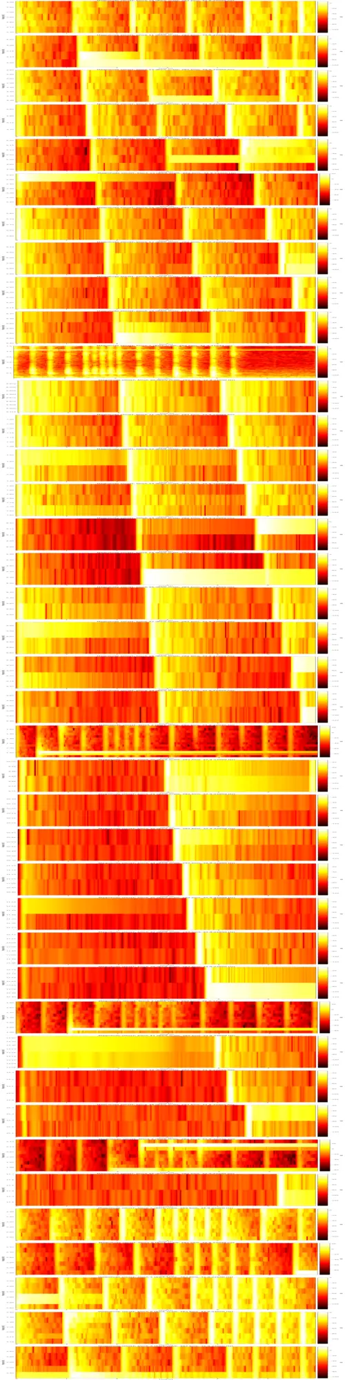

Resizing + stacking done with some simple cli tools:

mogrify -resize 500x50! plots/to-stack/*.png
convert -append plots/to-stack/*.png out.png

The key concept of xumx-sliCQ-V2 is that each of these distinct sub-spectrograms is operated on independently. That may also be a weakness, since the only knowledge the neural network has is constrained to the boundaries of each frequency block; no cross-block sharing.

Inference optimization (ONNX CPU)

I wanted to experiment with different inference optimization techniques. I was able to use ONNX on the default CPU provider to get a good speedup over the Torch model running on the CPU.

Step 1: load Torch model + params + sliCQT (NSGT in the code, but same thing):

# load model from disk
with open(Path(model_path, xumx_slicq_v2.json"), "r") as stream:
    results = json.load(stream)

# need to configure an NSGT object to peek at its params to set up the neural network
# e.g. M depends on the sllen which depends on fscale+fmin+fmax
nsgt_base = NSGTBase(
    results["args"]["fscale"],
    results["args"]["fbins"],
    results["args"]["fmin"],
    fs=sample_rate,
    device=device,
)

Step 2: get sample sliCQT from a waveform of seq_dur, which is the input to the NN:

nb_channels = 2
seq_dur = results["args"]["seq_dur"]

target_model_path = Path(model_path, f"{model_name}.pth")
state = torch.load(target_model_path, map_location=device)

jagged_slicq, _ = nsgt_base.predict_input_size(1, nb_channels, seq_dur)
cnorm = ComplexNorm().to(device)

nsgt, insgt = make_filterbanks(nsgt_base, sample_rate)
encoder = (nsgt, insgt, cnorm)

nsgt = nsgt.to(device)
insgt = insgt.to(device)

jagged_slicq_cnorm = cnorm(jagged_slicq)

xumx_model = Unmix(
    jagged_slicq_cnorm,
    realtime=not args.offline,
)

xumx_model.load_state_dict(state, strict=False)
xumx_model.freeze()
xumx_model.to(device)

Step 3: use sample input in the arguments to the ONNX export function:

dest_path = Path(model_path, f"{model_name}.onnx")

torch.onnx.export(
    xumx_model,
    (tuple([jagged_slicq_.to(device) for jagged_slicq_ in jagged_slicq]),),
    dest_path,
    input_names=[f"xcomplex{i}" for i in range(len(jagged_slicq))],
    output_names=[f"ycomplex{i}" for i in range(len(jagged_slicq))],
    dynamic_axes={
        **{f"xcomplex{i}": {3: "nb_slices"} for i in range(len(jagged_slicq))},
        **{f"ycomplex{i}": {4: "nb_slices"} for i in range(len(jagged_slicq))},
    },
    opset_version=16,
)

Note the use of dynamic axes for the slice dimension. For a given sliCQT and arbitrary waveform of length N, the resulting transform is of shape (batch, nb_channels, nb_f_bins, nb_slices, nb_t_bins). Each slice is a 2D "spectrogram", and consecutive slices are overlap-added. Every dimension except the slice is fixed and identical for any size of waveform.

• For the input, the fourth dimension (i.e. 3: "nb_slices") is slice: (batch, nb_channels, nb_f_bins, nb_slices, nb_t_bins)
• For the output, the fifth dimension (i.e. 4: "nb_slices") is slice: (batch, nb_targets, nb_channels, nb_f_bins, nb_slices, nb_t_bins), since all 4 target sliCQTs are returned in one tensor

I added opset_version=16 after researching some GitHub issues where, without setting this, the ONNX export was prohibitively slow (on the scale of hours).

From implementing the faster CPU inference (7s for a total song on average, vs 11s with Torch + CPU), I had the idea to create a Demix UI (user interface).

DemixUI

It's a graphical application using Kivy, and it uses the Python asyncio library to context-switch between the audio and graphics. I don't think asyncio is the right choice for any serious musical application, because here's the catch: the UI code is only run between each chunk that is demixed and streamed. So the responsiveness of the UI to human touch, or latency, is dependent on the music demixing latency! For a better design, it should probably be using multiprocessing (or multithreading), but I had no patience for figuring out how that works. I also thought the demix-latency-dependent UI is a funny aspect of the project (and it's a research toy anyway, so who cares?)

Screenshots:

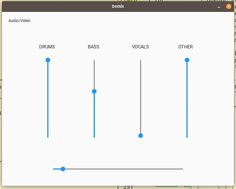
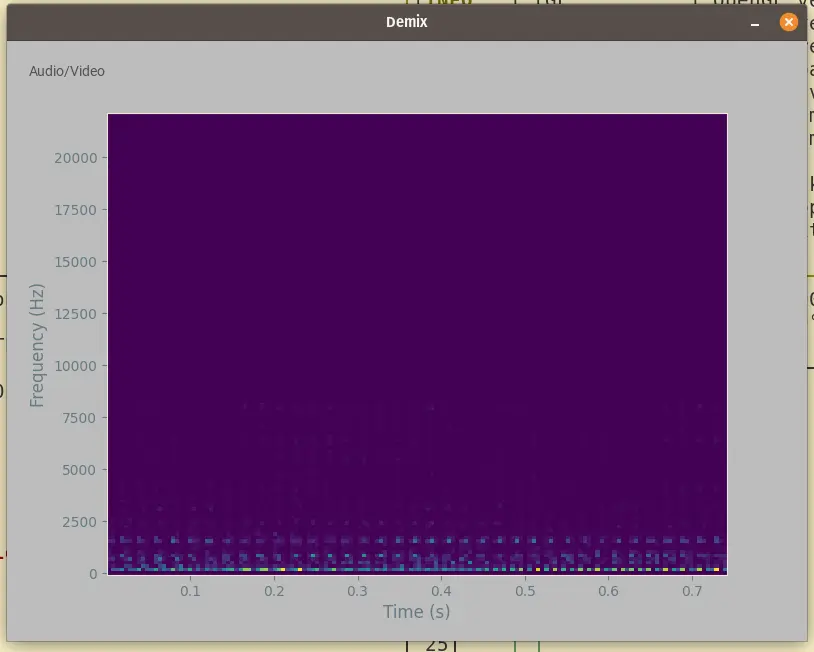
The Audio/Video is a toggle that displays the spectrogram of the demixed output (which is the audio being played).

The audio output stream size (using the torchaudio ALSA output stream on Linux, where the input is a wav file chunked into stream-sized tensors) is the next-largest-power-of-two of the sliCQT slice size. For a slice size of 18060 (for the default large offline and realtime models that use a 262-bin Bark scale from 32.9-22050 Hz), the next power of two is 32768 samples. Divided by a typical sampling rate of 44100 (what I use throughout xumx-sliCQ-V2), that represents 0.74s. The UI, then, will take roughly 0.74s to respond to any clicks and presses, which is actually horrible and feels very laggy and unresponsive.

For the smaller models, the sliCQT with a 32-bin Mel scale from 115.5-22050 Hz has a slice size of 2016 samples; the next power of two is 2048 samples. This is 0.0464s, or 46.4ms, which is much more reasonable and responsive as a UI latency. However, in this case, the demixing speed doesn't always keep up; the runtime of xumx-sliCQ-V2 doesn't always finish neatly within 46.4ms, leading to clicks from disjoint/slow output streams (if you've ever worked on a realtime audio output streaming project, clicks will be familiar).

So, the choices for DemixUI are:

• Good quality music demixing output, very slow (0.74s) UI/responsiveness
• Bad quality music demixing output, failed output quality, and faster UI/responsiveness at 46.4ms

Here's an example showing the asyncio code and why it behaves this way:

# run like so
$ python -m xumx_slicq_v2.demixui --input-file=./song.wav

# code
async def ui_code():
    kivy.run_app(): # or whatever
        # respond to user touches/inputs
        # update volume sliders for vocals, drums, bass, other

stream = StreamWriter(dst="default", format="alsa")
stream.add_audio_stream(44100, nb_channels)

# root is the kivy ui
async def demix_code(root):
    with stream.open():
        for frame, audio_chunk in enumerate(audio_chunks_iter):
            demixed = xumx_separator(audio_chunk)

            # get volume slider values from ui
            bass_level = root.bass_slider.value_normalized
            drums_level = root.drums_slider.value_normalized
            vocals_level = root.vocals_slider.value_normalized
            other_level = root.other_slider.value_normalized

            # adjust output mix dynamically based on sliders
            output_mix = other_level*demixed[0].T +
                bass_level*demixed[1].T + 
                vocals_level*demixed[2].T + 
                drums_level*demixed[3].T

            stream.write_audio_chunk(0, output_mix)

            # update the frame-by-frame progress slider
            root.update_slider(frame)

            # update the spectrogram
            root.update_spectrogram(get_spectrogram(output_mix, rate))

Unsuccessful changes

Most of these unsuccessful directions during the development of xumx-sliCQ-V2 are stored in a private archived repo: I might re-use them later, or I might not.

Any attempts encompassing neural network design (GRUs, LSTMs, interpolation of the ragged transform to make it square, and more) are omitted from this post. I'm happier to talk about the working version of xumx-sliCQ-V2 and bolted-on additions that I tried to make it better, rather than fundamental changes to the network architecture.

At the tail of end xumx-sliCQ (v1), I proposed some ideas that I predicted could improve the performance. The interpolated square matrix form is the most worthless one (and it makes the sliCQT computationally unfeasible by stuffing it with 0s and taking up so much space).

The ideas that were relevant and that I ended up using were:

• Eliminating the errors of the overlap-add procedure
• Using the complex MSE loss from Danna-Sep

The rest of these subsections describe the failed bolt-on improvements.

Blending models

At one point, I had models trained using different loss functions:

• MSE-only
• MSE + SDR
• SDR-only

I thought I could pick and choose the best model by blending the specific targets. The model blending code was fun to write, and helped cement my knowledge of my own model and how to navigate its different corners using PyTorch. However, the outcome wasn't worth it. Since I leapfrogged the performance gains later with more important changes, I got rid of the blending code as an unnecessary complication.

First, my different models were loaded using command-line flags:

$ python -m xumx_slicq_v2.evaluation --model-path=pretrained_models/mse
$ python -m xumx_slicq_v2.evaluation --model-path=pretrained_models/mse_sdr
$ python -m xumx_slicq_v2.evaluation --model-path=pretrained_models/sdr

The blending code would load my handpicked models and blend the weights of each that excelled in the evaluations:

print("Blending MSE + MSE-SDR models...")

mse_model_path = "/xumx-sliCQ-V2/pretrained_model/mse"
mse_model_path = Path(mse_model_path)

# when path exists, we assume its a custom model saved locally
assert mse_model_path.exists()

mse_xumx_model, _ = load_target_models(
    mse_model_path,
    sample_rate=44100.,
    device=device,
)

msesdr_model_path = "/xumx-sliCQ-V2/pretrained_model/mse-sdr"
msesdr_model_path = Path(msesdr_model_path)

# when path exists, we assume its a custom model saved locally
assert msesdr_model_path.exists()

msesdr_xumx_model, _ = load_target_models(
    msesdr_model_path,
    sample_rate=44100.,
    device=device,
)

# copy bass cdae from mse-sdr model into mse model
print("Deep-copying single cdae from mse-sdr model into mse model")

for i in range(len(mse_xumx_model.sliced_umx)):
    sliced_obj = mse_xumx_model.sliced_umx[i]

    if type(sliced_obj) == _SlicedUnmix:
        # second-last cdae i.e. index 2 is the 'other' cdae
        mse_xumx_model.sliced_umx[i].cdaes[2] = copy.deepcopy(
                msesdr_xumx_model.sliced_umx[i].cdaes[2])

blend_model_path = "/xumx-sliCQ-V2/pretrained_model/blend"
blend_model_path = Path(blend_model_path)

print("Now saving blended model")
torch.save(
    mse_xumx_model.state_dict(),
    Path(blend_model_path / "xumx_slicq_v2.pth")
)

I believe this change got me from 4.1 dB to 4.16 dB. Generally when people talk about blending models, they blend several top-performing SOTA (state-of-the-art) models to get a world-beating solution within a single competition in Kaggle. In my case, I applied blending privately to blend different trained variants of xumx-sliCQ-V2, so that the whole mess was still focused on my own ideas.

Pruning weights

Like blending models, I heard of "pruning weights" and thought I could use it for some benefits. PyTorch has some pruning functionality, but the kicker is that when the weights are pruned (and those tensors are zeroed), the raw .pth file doesn't get any smaller unless you apply gzip compression.

Let's say that indeed I wanted the several-MB of space savings from a gzipped .pth.gz model (that can be un-gzipped on load, so it's still possible to pretend it's beneficial to download speeds or something; smaller is always better...).

I tried three approaches to pruning:

1. Train -> evaluate -> prune -> evaluate (i.e. just try my luck and see what happens)
2. Train -> evaluate -> fine-tune + prune loop (i.e. prune and only save if improved on the training/validation set); also called fine-pruning by some blog posts
3. Train + prune during training

None of them resulted in a better final SDR score on the test set of MUSDB18-HQ (although some exhibited better validation loss).

Here are some examples of my pruning code.

This is strategy #2, or "fine-pruning":

$ cat xumx_slicq_v2/pruning.py

import torch.nn.utils.prune as prune

...

# test pruning 10%, 20%, 30%, 40%, and 50% of weights
prunes_to_test = [0.1, 0.2, 0.3, 0.4, 0.5]

t = tqdm.tqdm(prunes_to_test, disable=args.quiet)
sub_t = tqdm.trange(1, args.finetune_epochs + 1, disable=args.quiet)

for prune_proportion in t:
    # create a new unpruned unmix; save last pruning if it was good
    unmix = copy.deepcopy(unmix_orig)

    t.set_description("Pruning Iteration")
    # unmix is blocked per-frequency bin

    prune_list = []

    # target upper frequency blocks to have less impact
    for target in range(4):
        for frequency_bin in range(3*n_blocks//4, n_blocks):
            base = f"sliced_umx.{frequency_bin}.cdaes.{target}"
            print(f"pruning {100*prune_proportion:.1f}% from submodule: {base}")

            # prune each layer
            prune_list.extend([
                f"{base}.0", # encoder 1 conv
                f"{base}.1", # encoder 1 batch norm
                # 2 is the relu
                f"{base}.3", # encoder 2 conv
                f"{base}.4", # encoder 2 batch norm
                # 5 is the relu
                f"{base}.6", # decoder 1 conv transpose
                f"{base}.7", # decoder 1 batch norm
                # 8 is the relu
                f"{base}.9", # decoder 2 conv transpose
                # 10 is the sigmoid
            ])

    for prune_name in prune_list:
        module = unmix.get_submodule(prune_name)
        if isinstance(module, nn.batchnorm2d):
            prune.l1_unstructured(module, name="weight", amount=prune_proportion)
            prune.remove(module, 'weight')
        elif isinstance(module, (nn.conv2d, nn.convtranspose2d)):
            prune.ln_structured(module, name="weight",
                amount=prune_proportion, n=2, dim=0)
            prune.remove(module, 'weight')

    # fine tune
    for epoch in sub_t:
        sub_t.set_description("fine-tune epoch")

        train_loss = loop()
        sub_t.set_postfix(train_loss=train_loss)

        # check result
        valid_loss = loop()
        sub_t.set_postfix(val_loss=valid_loss)

        es.step(valid_loss)

        if valid_loss == es.best:
            print(f"achieved best loss: {valid_loss}, saving pruned model...")
            pruned_pth_path = os.path.join(target_path, "xumx_slicq_v2_pruned.pth")
            gz_path = os.path.join(target_path, "xumx_slicq_v2_pruned.pth.gz")
            torch.save(unmix.state_dict(), pruned_pth_path)

            # save as gzip; pruning + compression works best...
            with open(pruned_pth_path, 'rb') as f_in, gzip.open(gz_path, 'wb') as f_out:
                shutil.copyfileobj(f_in, f_out)

            # remove pruned pth file
            os.remove(pruned_pth_path)

            # base on best pruned model going forward; otherwise discard failed pruning
            unmix_orig = copy.deepcopy(unmix)

In pseudocode, what this does is:

1. Test out all those prune percentages (10%, 20%, 30%, 40%, 50%) one at a time
2. Apply those to the upper 75% of frequency bins; my assumption is higher frequency bins have more useless weights than lower frequency bins, given their higher time resolution (and thus more weights/bigger networks), while speech and music (and human hearing) contain important information generally in the lower frequency regions
3. Apply fine-tuning iterations where models that improved on the validation loss of the pretrained model are saved as a gzipped weights file

There are so many dimensions to this: which layers to apply pruning on (which depends more on my knowledge of xumx-sliCQ-V2 or convolutional autoencoders than any generalized pruning knowledge), whether to use L1 or LN pruning, structured pruning, unstructured pruning. It's hard to call this anything but "baby's first attempt to prune a model without understanding much about it at all." However, it was still worth a try, because models to tend to be sparse (i.e. the useful parts are accomplished by less than the full amount of weights).

My next approach, pruning-while-training (strategy #3), was kinda hilarious: at the end of each training iteration, randomly zap 1% of weights. This has a compounding effect (remove 1% of the weights i.e. preserve 99% of the weights, then 1% of that i.e. 99% of 99%, etc.) Also, bad end results. Not worth it.

# end of training - update tensorboard, apply pruning

train_times.append(time.time() - end)

if tboard_writer is not None:
    tboard_writer.add_scalar(f"Loss/train (MSE)", train_loss, epoch)
    tboard_writer.add_scalar(f"Loss/valid (MSE)", valid_loss, epoch)

if args.prune:
    _l1_prune_unmix(unmix, args.prune_per_epoch, n_blocks)


...

def _l1_prune_unmix(unmix, prune_proportion, n_blocks):
    # target upper frequency blocks to have less impact
    prune_list = []
    for target in range(4):
        for frequency_bin in range(n_blocks):
            base = f"sliced_umx.{frequency_bin}.cdaes.{target}"
            print(f"pruning {100*prune_proportion:.1f}% from submodule: {base}")

            # prune each layer
            prune_list.extend([
                f"{base}.0", # encoder 1 conv
                f"{base}.1", # encoder 1 batch norm
                # 2 is the relu
                f"{base}.3", # encoder 2 conv
                f"{base}.4", # encoder 2 batch norm
                # 5 is the relu
                f"{base}.6", # decoder 1 conv transpose
                f"{base}.7", # decoder 1 batch norm
                # 8 is the relu
                f"{base}.9", # decoder 2 conv transpose
                # 10 is the sigmoid
            ])

    for prune_name in prune_list:
        module = unmix.get_submodule(prune_name)
        if isinstance(module, nn.BatchNorm2d):
            prune.l1_unstructured(module, name="weight",
                amount=prune_proportion)
            prune.remove(module, 'weight')
        elif isinstance(module, (nn.Conv2d, nn.ConvTranspose2d)):
            prune.ln_structured(module, name="weight",
                amount=prune_proportion, n=1, dim=0)
            prune.remove(module, 'weight')

Note that the pruning code has the same challenges as the fine-pruning code: what layers to prune and how is a deep topic and it's hard to say whether this one single failure of mine invalidates pruning as a strategy.

However, by this point I gave up on the idea that I would beat 4.4 dB by deleting weights; and since beating 4.4 dB was my entire goal, I eliminated the complication of pruning from the project. Still, I tried.

Frequency scales: STFT <-> Multiresolution STFT <-> sliCQT

The sliCQT/NSGT give you the ability to create a time-frequency transform with an arbitrary nonuniform frequency scale. However, they can also be used to create a linear or uniform frequency scale. The sliCQT with a single fixed Q-factor and the even frequency spacing (df) of the STFT will boil down to the STFT! The list of ragged time-frequency blocks will be a list of one tensor, and that one tensor will resemble the STFT exactly (frames, frequency bins, etc.).

Imagine a sliding scale with the STFT on one-side (linear/uniform) and some "extreme" amount of nonuniformity/nonlinear/raggedness on the other:

STFT, linear |---------------------| sliCQT, nonlinear

The sliCQT can be used to implement any of them. Therefore, xumx-sliCQ-V2, with a uniform STFT frequency scale, boils down to a traditional STFT-based neural network!

A multiresolution STFT can be implemented with the sliCQT. Imagine the following:

• You want frequencies 0-100 Hz analyzed with an STFT with a window size of 16384 (very long windows, for bass notes)
• You want 100-400 Hz analyzed with 8192
• You want 400-800 Hz analyzed with 4096
• etc.

This is all achievable with the sliCQT. However, when it came down to working on xumx-sliCQ-V2 and preserving the same neural network (convolutional denoising autoencoder) and substituting the original Bark scale with the Linear STFT scale or arbitrary Multiresolution STFT scale, the results were again not great.

A different approach from the ground up might do this:

• Use the sliCQT to implement UMX (open-unmix) exactly the way it already is (using the STFT with window size 4096)
• Then slightly and cautiously, based on empirical measurements, alter the sliCQT to introduce different nonuniform frequency scales, while adapting the network architecture, until good results are reached
  • It's already true that Open-Unmix has different performance characteristics per-target for different STFT window sizes, so maybe that information can be used to create multiresolution STFT frequency scales for the sliCQT

Extra data

Data is probably the most important part of a neural network. Lots of participants in the MDX 21 (and new SDX 23) challenges were incorporating extra datasets of music. I have access to two rather small extra datasets:

• One is from a joint project with a friend, the OnAir Music Dataset: the dataset consists of stems to the tracks provided by the project, whose goal is royalty-free copyright-free music for Twitch streamers
• One is a handful of Periphery (metal band) album stems that I purchased from their digital store

One of the tiny models in xumx-sliCQ-V2 is trained on Periphery (for realtime metal demixing). However, I didn't find a way to gain any hands-down dramatic increases in music demixing performance by incorporating the extra data.

I think, much like neural network design, although extra data matters, it must be done carefully: the data must be useful! And perhaps not conflicting. The screaming vocals of a metal band likely don't mix well with the pop vocals in MUSDB18-HQ in a way that helps xumx-sliCQ-V2 generalize, and the OnAir Music Dataset is most likely too small to make a real difference.

Throwing in random stems and hoping for the best is probably similar to how I threw in random network architecture changes and hoped for the best: low-percentage, shooting in the dark.

Training optimization: PyTorch 2.0

Right around when I was working on xumx-sliCQ-V2, PyTorch made its 2.0 announcement with the new torch.compile function that would make training faster. Sounds great! But it didn't work for xumx-sliCQ-V2. I don't have the exact stack trace but it's related to unsupported operators or modules deep in the network, and in a way that I continued with PyTorch 1.14 (supplied by the NVIDIA PyTorch container).

Inference optimizations: ONNX (CUDA, OpenVINO), TensorRT, Torchscript

I wanted to try fancier inference optimization techniques. The Torchscript export works relatively well, but to use it (in, say, a high-performance C++ app), I'd need a C++ implementation of the sliCQT.

I was able to implement the ONNX CUDA operator with improved data transfer characteristics by using io_binding to appropriately deal with host/device tensors. However, the ONNX CUDA inference speed was worse than regular Torch + CUDA. It could be an error in my use of io_binding, but I stuck with ONNX CPU.

Next, I tried ONNX's TensorRT backend: no luck. I also tried to use TensorRT directly, and that was tricky as well with the list-of-tensors input of the Unmix module. My last attempt was the ONNX OpenVino runtime, and even that gave me some errors. I stuck with the works-just-fine ONNX CPU vanilla platform for some solid gains.

I also tried to export the entire Separator model of xumx-sliCQ-V2, which performs the forward and backward sliCQT operation, and takes a waveform as an input. This would give me an entire compiled module (with Torchscript, TensorRT, ONNX, etc.), and remove the need to even think about reimplementing the sliCQT. However, again, these complicated forward and backward transforms couldn't be compiled to ONNX (FFT/iFFT not supported yet).

Conclusion: closing the loop on many ideas

It's been a few years that I've been focused on music-related code.

In Real-Time-HPSS, I experimented with applying Harmonic/Percussive Source Separation (HPSS) in a realtime loop. Zen is a high-performance C++/CUDA implementation of the same idea.

In Music-Separation-TF, I did a lot of experiments with spectrogram masking and different nonlinear time-frequency transforms, focusing on the harmonic/percussive (or tonal/transient) idea. During that time, I discovered the NSGT and also created my first music demixing neural network from scratch, MiXiN, which measured up badly to UMX.

In headbang.py, I tried to crack the secret to what makes a song groove and make metal fans want to bang their heads. I applied a combination of Harmonic/Percussive Source Separation and transient shaping to sharpen percussive onsets before feeding the separated waveforms to ensemble beat tracking and onset detection algorithms. I abandoned beat tracking when I learned that beats are ambiguous, subjective, and depend on the annotator.

In xumx-sliCQ, I tried to create a proper music demixing system with SOTA performance by using the sliCQT in X-UMX. I worked on this during the 2021 Music Demixing Challenge, and managed to produce a decent PyTorch port of the original NumPy NSGT/sliCQT library. I was swept up in the world of music demixing, and worked with a friend to publish the OnAir Music Dataset to (try to) help advance research in the domain.

xumx-sliCQ-V2 is a continuation of all of these ideas. I tried to make it realtime with the proposed network architecture variant. I tried to make it fast with ONNX and TorchScript, to use in C++ applications. I tried to apply it as a preprocessing step before the ensemble algorithms of headbang.py to create an amazing beat tracker (spoiler: nothing good came of it). I tried to use my extra data to improve its generalization performance.

xumx-sliCQ-V2 is OK. Good, not great.

The highlights are the development/REPL loop with Docker and the pure-convolutional architecture. Using Docker with volume mounts helps me deal with Python packaging in the best way possible, and it's finally a deep learning codebase I can walk away from and come back to without fuss (the commands Just Work(TM)). Absorbing the task of the overlap-add procedure into the convolutional layers also reduces the barrier to understanding the transform.

The lowlights are that again I performed a high effort/low quality kitchen sink approach to go from 3.6 dB to 4.4 dB, and I don't know if or when I'll ever be able to compete with the original X-UMX, let alone approach SOTA performance. There are too many dimensions to consider.

I don't know if xumx-sliCQ-V3 will be better (or if there will be one at all), but I don't give up easily.

Comments